You've read about TSP (ordering stops) and about VRPTW (respecting time windows). One very common practical case is left: you have multiple vehicles. 2 drivers in the morning, 5 caregivers in the field, 3 caterers heading out at the same time. How do you split customers between them to minimize total time?
That's the VRP (Vehicle Routing Problem) and the most used method in practice dates back to 1964: the Clarke and Wright Savings algorithm. That's what OptiRoad uses on its Business plan to handle 2 to 10 vehicles.
The problem in one sentence
You have 1 depot and N customers to deliver. You have M vehicles available. How do you split the N customers across the M vehicles so that total time is minimal?
Sounds simple. It isn't.
Why it's hard
With 20 customers and 3 vehicles, the number of possible partitions exceeds 3.5 million. And for each partition, you still need to solve a TSP (or VRPTW with time windows) on each vehicle. Brute force is impossible past 10 to 15 customers.
The VRP, like the TSP, is NP-hard: no algorithm guarantees the optimal solution in reasonable time. So we use heuristics. The one that has dominated real-world use for 60 years is Clarke-Wright Savings.
Clarke-Wright's brilliant idea (1964)
George Clarke and John Wright published their paper "Scheduling of vehicles from a central depot to a number of delivery points" in 1964. The idea is disarmingly elegant.
Step 1: the naive solution
Start with a degenerate solution: each customer has their own vehicle. 20 customers = 20 mini-routes depot → customer → depot. Wasteful, but it's our starting point.
Total cost: for each customer i, the vehicle does d(depot, i) + d(i, depot) = 2 × d(depot, i).
Step 2: the "saving" concept
Imagine merging the routes of two customers i and j into a single one. Instead of:
depot → i → depot + depot → j → depot
You do:
depot → i → j → depot
The saving is:
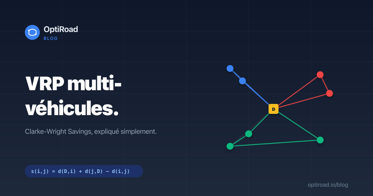
s(i,j) = d(depot, i) + d(j, depot) - d(i, j)
The closer i and j are to each other and the further from the depot, the larger the saving. Intuitive: it's worth grouping them.
Step 3: greedy merging
- Compute s(i,j) for all pairs of customers
- Sort these savings in descending order
- For each pair (i,j), in order:
- If i and j are on different routes
- And they're at the extremities of their respective routes
- And we still have vehicles available (≤ M)
- Merge the two routes
- Continue until no useful pairs remain
At the end, you get M routes (or fewer) that cover all customers, with a total distance much better than the naive solution, typically within 5 to 10% of the theoretical optimum.
Savings, sweep or metaheuristic?
Clarke-Wright is not the only family of algorithms for the VRP. Three broad approaches coexist.
The sweep algorithm (Gillett and Miller, 1974) groups customers by their angle around the depot, like a clock hand sweeping across the plane. It is extremely simple to code, but the route quality stays lower: you follow the geometry, not the real cost.
Metaheuristics (tabu search, genetic algorithms) explore the solution space more thoroughly and reach slightly better results. The trade-off is that they are slower and trickier to tune: you have to calibrate many parameters, which makes them heavy to put into production.
Clarke-Wright Savings sits at the ideal sweet spot: near-optimal results, fast execution, rock-solid robustness, and an easy path to extend it with capacities or time windows. That is exactly why it has dominated real-world fleet routing for 60 years.
A concrete example
Picture 6 customers to deliver from a Paris-center depot, with 2 vehicles available:
| Customer | Distance to depot |
|---|---|
| A | 4 km |
| B | 5 km |
| C | 8 km |
| D | 6 km |
| E | 9 km |
| F | 7 km |
Naive solution (1 vehicle per customer, 6 vehicles):
- Total cost: 2 × (4 + 5 + 8 + 6 + 9 + 7) = 78 km
With Clarke-Wright Savings and 2 vehicles:
- Compute savings for the 15 possible pairs
- Sort descending
- Successive merges respecting the 2-vehicle cap
- Possible result: Vehicle 1 =
depot → A → B → D → depot(~22 km), Vehicle 2 =depot → C → F → E → depot(~28 km)
- Total cost: ~50 km (-36% vs naive)
On real cases, gains of 30 to 40% over a manual "by-eye" partition are common.
Variants and extensions
The original algorithm is for the basic VRP. In practice, we enrich it:
- Capacities: each vehicle has a max load. We check on each merge that we don't exceed capacity.
- Multi-depot: several depots. Heuristic: assign each customer to the closest depot, then Clarke-Wright on each sub-problem.
- Time windows: combine with VRPTW. Only merge two routes if the resulting order respects all windows.
- Bound on vehicle count: if you want exactly M vehicles, stop merging earlier.
- Asymmetry: distance A→B can differ from B→A (one-way streets, etc.). The savings calculation remains valid.
How OptiRoad implements multi-vehicle VRP
On the Business plan, you can optimize up to 10 vehicles in parallel. Here's what OptiRoad does when you enable multi-vehicle mode:
- Configuration: you set the vehicle count, their depot (shared or per-vehicle), and optionally their arrival point.
- Clarke-Wright Savings: compute savings on all pairs, sort descending, greedy merges respecting the vehicle cap.
- Multi-depot: if each vehicle has a different depot (
sharedDepot: false), pre-assign stops by proximity before running Clarke-Wright on each cluster. - Per-vehicle local TSP: once the partition is found, each route is re-optimized individually with nearest neighbor + 2-opt to minimize internal distance.
- If VRPTW is active: EDF (Earliest Deadline First) on each route, respecting each customer's time windows.
- Distinct colors: each vehicle gets a color on the map (#3B82F6, #EF4444, #10B981, etc.) for easy route visualization.
Adaptive timeouts: 15 seconds for 2 to 4 vehicles, 30 seconds for 5 to 10 vehicles. If exceeded, OptiRoad returns the best result found with a partial: true flag.
Drag and drop for manual adjustments
If the automatic split doesn't suit you (a customer absolutely must be assigned to a specific driver for client-relationship reasons), you can drag and drop a stop from one vehicle to another in the app. OptiRoad then recomputes the TSP order for each impacted vehicle while respecting the new partition. Endpoint: POST /api/optimize/reorder (Business plan only).
Balancing the routes
In its raw form, Clarke-Wright chases one thing only: minimizing total distance. As a result, it can produce unbalanced routes, one driver loaded with 25 stops while another has just 8. On paper the distance is optimal; in real life that's unworkable for planning.
In practice, you therefore cap the number of stops or the capacity per vehicle to force a more even split. Then you rebalance by hand when the field demands it. OptiRoad lets you fix the number of vehicles and move stops from one to another via drag and drop: each affected route is recomputed instantly, so you keep an optimized order while staying in control of each driver's load.
When to use multi-vehicle
- 2 to 3 vehicles: useful as soon as your day exceeds 30 stops, or you deliver to distinct geographic zones.
- 5 to 10 vehicles: for structured fleets (home care, caterers with a team, scaling e-commerce).
- Beyond 10 vehicles: contact us, we can enable a dedicated solver for very large fleets.
In practice: what it changes for you
On a typical day of 60 deliveries to split across 3 drivers:
- Without optimization (rough manual split): ~280 km, 12 cumulative hours
- With OptiRoad's Clarke-Wright Savings: ~190 km, 8 cumulative hours
- Gain: -32% distance, -33% cumulative time
Beyond kilometres, the real win is organizational: each driver starts with a clean route sheet, their color on the map, precise ETAs. No more "who takes who?" in the morning.
Going further
Multi-vehicle VRP is exclusive to the Business plan (€49/month). The Pro plan stays single-vehicle (with or without time windows).
This 3-article series (TSP → VRPTW → multi-vehicle VRP) covers the conceptual foundations of OptiRoad. Future articles will tackle practical topics: real savings, integrating the API with your e-commerce store, and more.
FAQ
How many vehicles does OptiRoad handle? From 2 to 10 vehicles on the Business plan. Beyond that, contact us: we can enable a dedicated solver for very large fleets.
Can each vehicle have a different depot? Yes, multi-depot mode is built for that. Stops are pre-assigned to the nearest depot before Clarke-Wright runs on each cluster, which guarantees consistent routes per zone.
Can I lock a customer to a specific vehicle? Yes, with drag and drop. You move the stop to the vehicle you want and OptiRoad immediately recomputes the TSP order of the affected vehicles to keep every route optimized.
Which plan is required? The Business plan only. The Pro plan stays single-vehicle, with or without time windows.