If you deliver to 15, 30 or 100 customers a day, you've already been doing TSP without knowing it: the Traveling Salesman Problem. It's one of the most studied problems in computer science, and it's exactly what OptiRoad solves every time you hit "Optimize". This guide explains in plain words what it is, why it's harder than it looks, and how it's solved in practice.
The problem, in one sentence
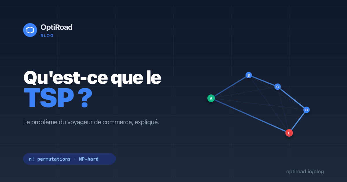
You have a starting point (your depot, your home) and a list of addresses to visit in a day. What's the visit order that minimizes total distance traveled? That's the TSP.
Trivial to state, brutally hard to solve once you go past a dozen addresses. This is exactly where human intuition runs out of road: the eye can spot a good 5-stop route easily, a good 40-stop route far less so. What sounds like a small detail (which order do I drive in?) actually decides a large share of your daily driving time and your costs.
A concrete example
Imagine 5 deliveries in Paris:
- A: République
- B: Bastille
- C: Montparnasse
- D: Étoile
- E: Pigalle
If you start from your depot and go in alphabetical order A → B → C → D → E, you'll most likely zigzag across town. In practice, that alphabetical route sends you from the east of Paris over to the west and back: count roughly 13 km. By reorganizing the same 5 addresses intelligently (for example by grouping the stops that sit close together), the optimized order drops to about 9 km, roughly 30% less for the exact same deliveries. Over 200 working days a year, those per-route savings add up to thousands of kilometres, meaning hours of driving and a meaningful fuel budget.
Why the TSP is hard
With 5 addresses, there are 5! = 120 possible orderings. A human can test them by hand. With 10 addresses, that climbs to 3.6 million orderings. With 20, it's 2.4 quintillion. No computer in the world can test every combination of a 30-stop route in a reasonable time.
The TSP is NP-hard: no known algorithm can guarantee the perfect solution in a time that scales reasonably with the number of stops. Every address you add multiplies the search space rather than just adding to it.
Key takeaway: for 10 addresses or fewer, you can still test every combination and guarantee the absolute optimum. Beyond that, we use heuristics, strategies that give a very good solution without guaranteeing mathematical perfection.
A bit of history
The TSP is not new. Mathematicians have been studying it since the 1930s: the Austrian mathematician Karl Menger discussed it in Vienna within his scientific circle, and the problem soon spread to American universities. The turning point came in the 1950s at the RAND Corporation, where George Dantzig, Delbert Ray Fulkerson and Selmer Johnson published in 1954 the exact solution to a famous instance: an optimal tour linking 49 cities of the United States (one per state, plus Washington). It was a remarkable feat for the time, achieved with linear programming methods and a great deal of hand computation. Even today, the TSP remains a reference benchmark in operations research and logistics: new algorithms are often measured against these historic instances.
Approaches in practice
1. Brute force (≤ 10 stops)
Test every possible permutation, keep the best. Guarantees the absolute optimum but becomes impractical past 10 stops.
2. Nearest neighbor (simple heuristic)
At each step, go to the closest remaining stop. Fast, but often far from optimal: you can end up stranded far from the rest of the stops.
3. 2-opt (local improvement)
Start from an initial solution (often from nearest neighbor), then try to "untangle" crossings by reversing route segments. Iterative, typically delivers results within 5% of the theoretical optimum.
4. More advanced algorithms
Lin-Kernighan, simulated annealing, genetic algorithms, constraint programming: many approaches exist in operations research. They can squeeze out the last bit of accuracy, but they are more complex to implement and maintain. For business use cases like delivery, nearest neighbor + 2-opt strikes the best balance of simplicity, quality and speed: easy to reason about, very fast, and close to optimal on real routes.
Perfect optimum, or very good right now?
This is the real question when you design a delivery tool. A solver can aim for the mathematically perfect solution, but that can take hours of computation on a large route. Out in the field, though, nobody waits hours to set off. A solution within a few percent of optimal, computed in seconds, easily beats a perfect solution that arrives too late.
Why? Because the last few percent of distance shaved off are almost never worth the wait: between a 9.0 km route and an 8.8 km route, the difference across your day is negligible, while the computation time can explode. That is exactly why heuristics like nearest neighbor + 2-opt are the right engineering choice: they deliver the bulk of the gain, immediately and reliably. Theoretical perfection is a matter for researchers; daily profitability is a matter for drivers.
The variants that matter for delivery
The "pure" TSP assumes you return to the starting point. In practice, your constraints are richer:
- Open-loop TSP: no return to depot (you end at the last customer).
- VRPTW (Vehicle Routing Problem with Time Windows): each address has an opening time range (e.g. 9am to noon). This is what you use for delivery time windows.
- Multi-vehicle VRP: multiple drivers, so how do you split stops across vehicles to minimize total time?
- Capacitated VRP: each vehicle has a maximum payload.
OptiRoad handles these variants: VRPTW for time windows (Pro and Business plans) and multi-vehicle VRP with the Clarke-Wright Savings algorithm (Business plan, up to 10 vehicles).
How OptiRoad solves your TSP
Every time you click Optimize in the dashboard, OptiRoad runs the following pipeline:
- Geocodes your addresses (turns them into GPS coordinates) if they aren't already.
- Builds the distance matrix between all points via OpenRouteService (or Google Routes as fallback).
- If ≤ 10 stops: brute force, every permutation tested, absolute optimum guaranteed.
- Otherwise: nearest neighbor to build the initial route, then 2-opt to refine through successive iterations.
- If VRPTW is enabled: the solver respects time windows via an Earliest Deadline First approach, flagging any predicted lateness.
- If multi-vehicle: Clarke-Wright Savings to split stops, then local TSP on each route.
All of this in seconds (3 seconds for 15 stops, up to 20 seconds for 150 stops with adaptive timeout).
In practice: what it changes for you
On a typical 30-delivery urban route:
- Without optimization: about 120 km, about 5 hours on the road
- With OptiRoad: about 85 to 90 km, about 3.5 to 4 hours on the road
- Typical gain: 25 to 30% distance, 20 to 30% time
Over 200 working days a year, that's thousands of kilometres and hundreds of hours saved. All of it from solving a problem that has been called "the TSP" since 1930.
Frequently asked questions
How many addresses can OptiRoad optimize?
Up to 150 stops per route. Up to 10 stops, brute force tests every combination and guarantees the absolute optimum. Beyond that, OptiRoad switches to heuristics (nearest neighbor, then 2-opt) that stay excellent even on large routes.
Is the route always the shortest possible?
Yes, and it is mathematically guaranteed up to 10 stops. Beyond that, the result typically lands within about 5% of the theoretical optimum thanks to 2-opt: a gap you won't notice in the field, for a near-instant computation.
Do I need a starting point?
Yes. You need a starting point: a depot or a home address. The end point, on the other hand, is optional: if you don't set one, OptiRoad assumes you return to your starting point (a round trip).
How long does the computation take?
A few seconds. OptiRoad uses an adaptive timeout: about 3 seconds for small routes, up to 20 seconds for 150 stops. If the limit is reached, the tool still returns the best route found. In practice, you have your finished order ready before you've even started the engine.
Going further
If you want to see the algorithm at work on your own addresses, the OptiRoad Free plan includes 5 routes a month with up to 10 stops, exactly the zone where brute force guarantees the absolute optimum. It's the best way to measure concretely what you'll save.
Want to dig into the variants (time windows, multi-vehicle)? Keep reading the other blog posts or check the API documentation.